The MSIM Quantitative Duration Strategy Model: A Factor-Based Approach to Managing Interest Rates

05 AUGUST 2026

The Authors

Top

Download

We use quantitative tools to enhance our investment process, as they help provide structure and rigour with identifying and processing relevant and important data.

Our proprietary MSIM Quantitative Duration Strategy (QDS) model advises us on tactical duration risk positioning in developed government bond markets. The model is based on five signals, which reflect factors we think are important:

Market Technicals
Risk Sentiment
Business Cycle
Carry
Valuation

These signals incorporate both fundamental and technical inputs based on the following criteria:

There is evidence that relationship has worked in the past.
Academic literature supports the idea of these inputs.
The relationship has a plausible fundamental or behavioural explanation.
Data is timely and readily available.
Signals have been additive to the performance of the strategy.

Individually, these signals have limited success in predicting bond returns vs cash (i.e., excess bond returns, which is the return one gets from taking duration risk), but when combined together they have created a more successful and reliable signal. This makes intuitive sense: by looking at a broader range of relevant data, one gets a better picture of the appropriate risk to take.

This strategy has generated attractive Sharpe ratios, resilient performances during periods of market stress and few significant drawdowns (before taking transaction costs into account). However, returns can be modest over extended periods, so the model should not be relied upon to deliver attractive results in all market conditions. QDS remains an important component of our investment process, but it is only one of several inputs we consider.

Introduction

Bond returns are highly sensitive to interest‑rate movements—i.e., duration risk—so managing that risk is critical, and effective management of this risk begins with understanding it. To that end, we have developed quantitative models that supplement our qualitative assessment of markets and provide a framework for quickly processing relevant information.

Changes in interest-rate levels are typically the primary source of risk for fixed-income portfolios, especially in government bonds and investment-grade credit. As a result, forecasting movements in bond yields is a core skill for fixed-income investors – even if, as the adage goes, making predictions, especially about the future, is very difficult.

From a fundamental perspective the challenge largely reduces to correctly anticipating central-bank policy. Because the central bank directly controls short-term rates, fluctuations at the front end of the curve tend to propagate to longer maturities. For example, changes in 12-month and shorter T-bill rates have historically explained 91% of the variation in 10-year U.S. Treasury (UST) yields^1¹. While past relationships are no guarantee of future outcomes, knowing the likely path of policy rates should, in principle, allow for robust forecasts of yields across the curve. This explains fixed-income investors’ intense focus on every nuance of central-bank communication and policy action.

But knowing that central-bank policy matters does not make the task much easier: forecasting it is formidable. It requires understanding the bank’s reaction function and the ability to forecast the inputs to that function – effectively, accurate macroeconomic forecasting. Moreover, getting the policy call right is sometimes insufficient. Yields can be decomposed into rate expectations (the average expected path of short-term policy rates) and the term premium (the additional yield investors demand for holding longer-maturity bonds rather than cash). Movements in the term premium can overwhelm the path of expected short rates, complicating yield forecasts across the curve.

Fortunately, there are other ways to forecast near-term interest-rate returns. Many are little more than common-sense rules of thumb about how markets behave in specific environments, but, taken together, they form a powerful and reliable framework for managing duration risk. Most of these rules are well documented in the academic literature; while we are not unique in using them, we do so with the confidence that they have been rigorously examined – by us and by many others. Moreover, we find that the same factors work well across all G7 government bond markets (indeed, in every market to which we have applied the analysis). This broad portability strengthens our conviction and provides a practical tool for guiding our duration positioning within and across markets.

QDS integrates a set of measurable market pricing factors that we have rigorously tested for their predictive power in forecasting future rate moves. We use the QDS signal – alongside our other quantitative and fundamental frameworks – to challenge and validate our investment thesis. The strength of these signals helps calibrate the timing and sizing of portfolio duration adjustments.

Adopting this process helps us in our goals to create alpha and achieve repeatable results in the duration management of portfolio.

MSIM Quantitative Duration Strategy (QDS) model

The model is based on five signals:

Market Technicals
Risk Sentiment
Business Cycle
Carry
Valuation

By considering a broader range of information, investors gain a clearer picture of the appropriate level of risk to take. Individually, these signals have limited ability to predict short-term excess returns, but when combined they generate a more robust and reliable signal. When all signals align in the same direction, it is logical to have greater conviction and undertake more risk; conversely, when the factors conflict, it is prudent to moderate active positions.

We find these signals work in all developed markets (DM). In addition, the relative scores between markets also provide useful positioning advice for trading cross market rates. However, while QDS has rarely gotten the markets very wrong (the model has had very few significant drawdowns), it has gone through long periods of low conviction and generating modest returns. So while QDS is an important part of our tool kit, it is not the only input in our interest rate decision-making process.

Factor-based approach
As noted earlier, the signals we use are either the same as, or closely related to, those documented in academic literature, so our approach is not necessarily novel. However, we find it reassuring that others have achieved success using similar methodologies. Our choice of inputs is guided not only by their historical effectiveness and intuitive appeal, but also by how they complement one another to create a stronger overall signal. In particular, we prioritise signals with low correlation to each other, as this increases the diversity of information within the signal.²

Signal 1: Market Technicals

QDS first signal is based on the average of two factors:

Momentum of returns – to gauge performance trend of duration.
Reversal – to measure tendency of rates to buck the trend.

MOMENTUM OF RETURNS
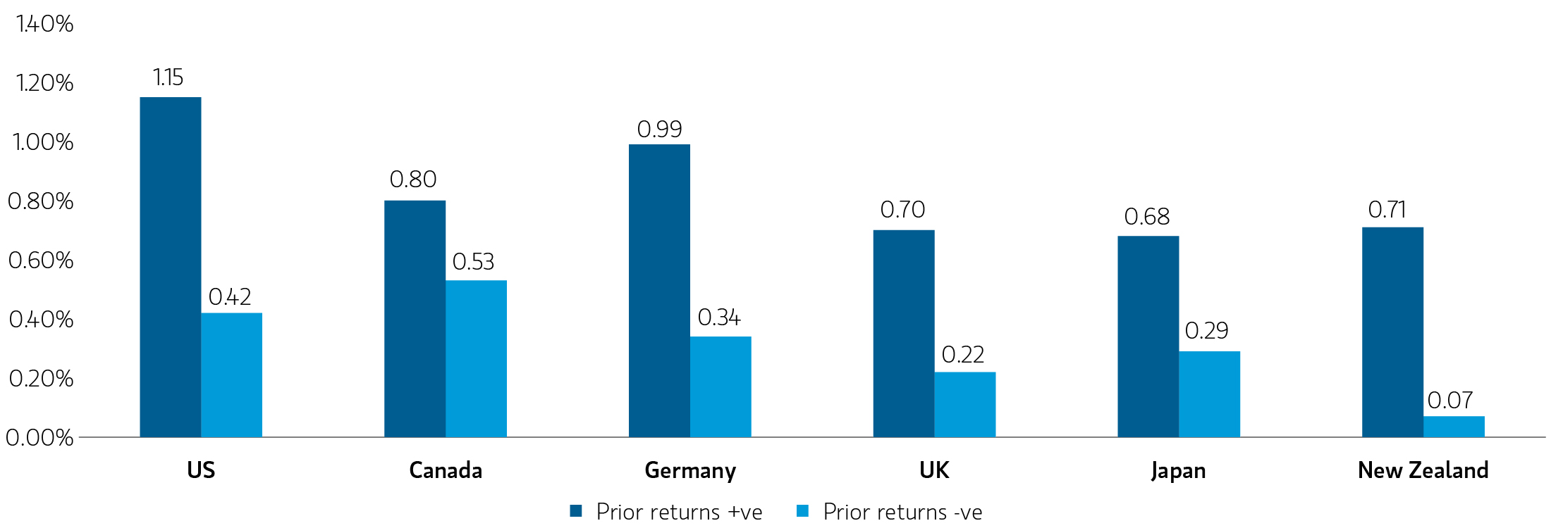
The old trader’s adage is that the trend is your friend: if asset prices are going up, they are more likely to carry on doing so, and vice versa. Momentum has been observed across multiple asset classes and is a popular signal in the factor investing approach. We find it works across most developed markets. For example, since 1997, if 10 year UST excess returns³ over the previous three months were positive, then subsequent returns were on average higher (1.15% annualised). On the other hand, if previous returns were negative, subsequent returns were lower (0.42%), if still positive. This pattern repeats across all the DM markets, Display 1, supporting the idea that it’s more attractive to be long government bonds if prior returns have been higher rather than lower⁴.

Display 1: Excess bond returns when prior 3 months were positive or negative

Source: MSIM, Bloomberg. Period of observation is from 1997-2025. The indexes are provided for illustrative purposes only and are not meant to depict the performance of a specific investment. Past performance is no guarantee of future results.

REVERSAL
Our second Market Technicals factor is Reversal. Rate markets - particularly developed‑market government bonds - are commonly used for portfolio hedging because they offer a liquid way to express a risk‑off view when investors expect drawdowns in higher‑beta holdings (e.g., equities, credit). Such portfolio hedging behaviour can cause government bonds to overshoot fundamentals. As a result, sharp moves in response to a risk shock are frequently reversed once the event has passed and pricing moves back towards fundamentals.

By explicitly capturing Reversal alongside Momentum, we build a more robust Market Technicals signal. Momentum recognizes the persistence of moves during trending regimes, while Reversal counterbalances it by identifying conditions where the probability of pullback is elevated (e.g., extreme positioning, stretched valuations, or sharp deviations from the mean). This pairing reduces the risk of chasing late‑stage trends, dampens whipsaw, and improves diversification across regimes – supporting more resilient allocation and hedging decisions.

Signal 2: Risk Sentiment

Our second signal is based on the average of two factors:

Momentum of equities returns - to gauge the performance of risky assets.
The Morgan Stanley Global Risk Demand Index – to capture broad risk-taking sentiment.

PRIOR EQUITY RETURNS
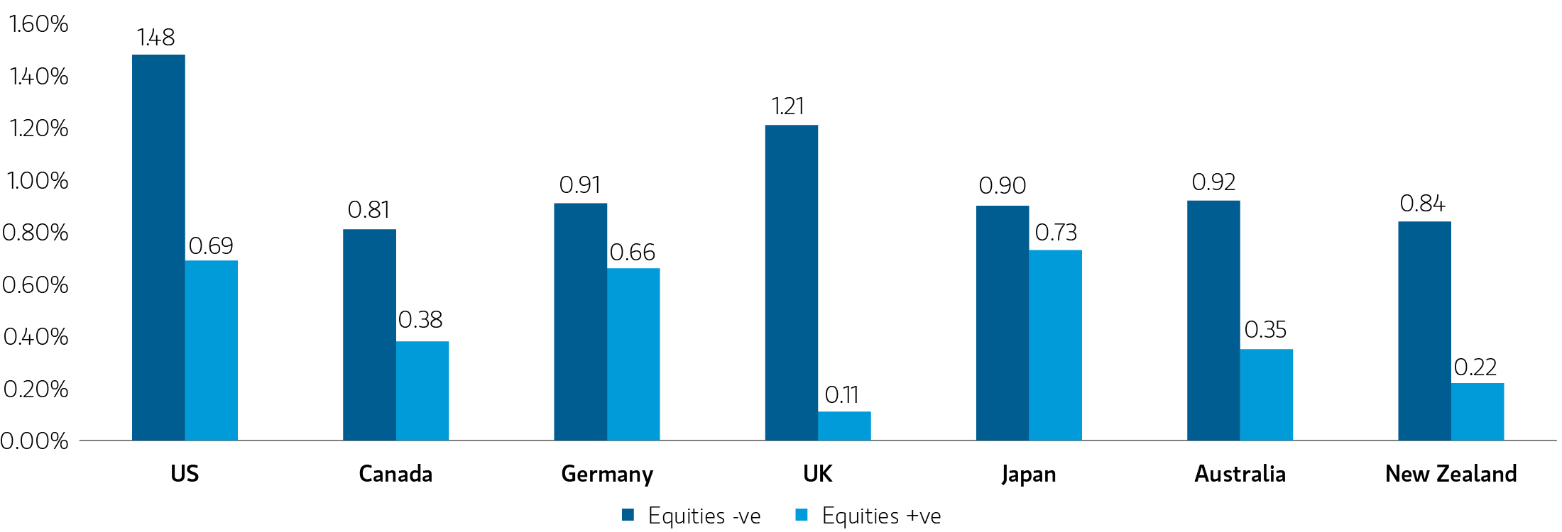
Across the major DM bond markets, we find that excess returns are higher when equity returns over the previous six months have been negative, and vice versa (Display 2). We also find the performance of emerging markets (EM) versus DM equity performance a useful indicator of future returns, i.e. bonds have done better when EM lagged behind, and vice versa. The idea that bonds should do well when equities do badly is not surprising, but what is interesting is that equity market performance tells us something useful about the potential for future bond market returns. One explanation for this is an “inverse wealth effect”: investors are more risk averse following a period of poor asset returns, which has reduced their net wealth⁵. This causes them to be more willing to buy government bonds. An alternative explanation is that there is persistence in asset price performance, which means past equity market returns are an indicator of future risk sentiment.

Display 2: Excess bond returns when prior equity returns were positive or negative

MORGAN STANLEY GLOBAL RISK DEMAND INDEX
Since 2004, Morgan Stanley has published a daily index measuring risk sentiment across markets.⁶ It combines 10 different asset classes into a single risk-taking measure, including volatility indicators of equity, bond and FX markets as well as performance of beta (EM vs G10 bonds, HY vs IG bonds, precious vs base metals, G10 equity vs bonds, growth vs value US equities).

The rationale behind the Risk Sentiment signal is that risk sentiment and the performance of risky assets tend to exhibit persistence, and equity market performance often has an inverse knock-on effect on risk-free assets like government bonds. Poor returns on risky assets reduce investor wealth, making investors more risk-averse and demanding higher allocation to rate products hence pushing risk free rates lower (and vice versa).

Signal 3: Business Cycle

The third signal comprises of two factors:

Economic surprises.
Commodity prices.

ECONOMIC SURPRISES
While it is natural for fixed‑income investors to track macroeconomic data because of its influence on monetary policy, the (generally) efficient pricing of new information suggests that the latest releases should not predict future returns, even when framed as surprises versus consensus. Yet our evidence shows that excess bond returns tend to be higher after downside surprises and lower after upside surprises.

COMMODITY PRICES
Commodity prices also carry useful information: higher commodity prices are typically negative for bond returns, likely via their impact on inflation and the monetary policy outlook, and because commodities often lead the business cycle. As with the signal we observe from equity market returns, the fact that past commodity moves help forecast bond return potential points to inefficiencies in how the bond market incorporates cross-asset information. Empirically, prior declines in commodity prices are associated with higher subsequent bond returns across the markets we have studied, a result that is also noted in the academic literature.⁷

Signal 4: Carry

The fourth rule is carry. It is generally better to be long duration when the yield curve is steep and carry is higher than when the curve is flat and carry is lower. Government bond investors earn carry both from receiving a bond yield above the cash rate and from roll‑down as their bonds move down the curve⁸.

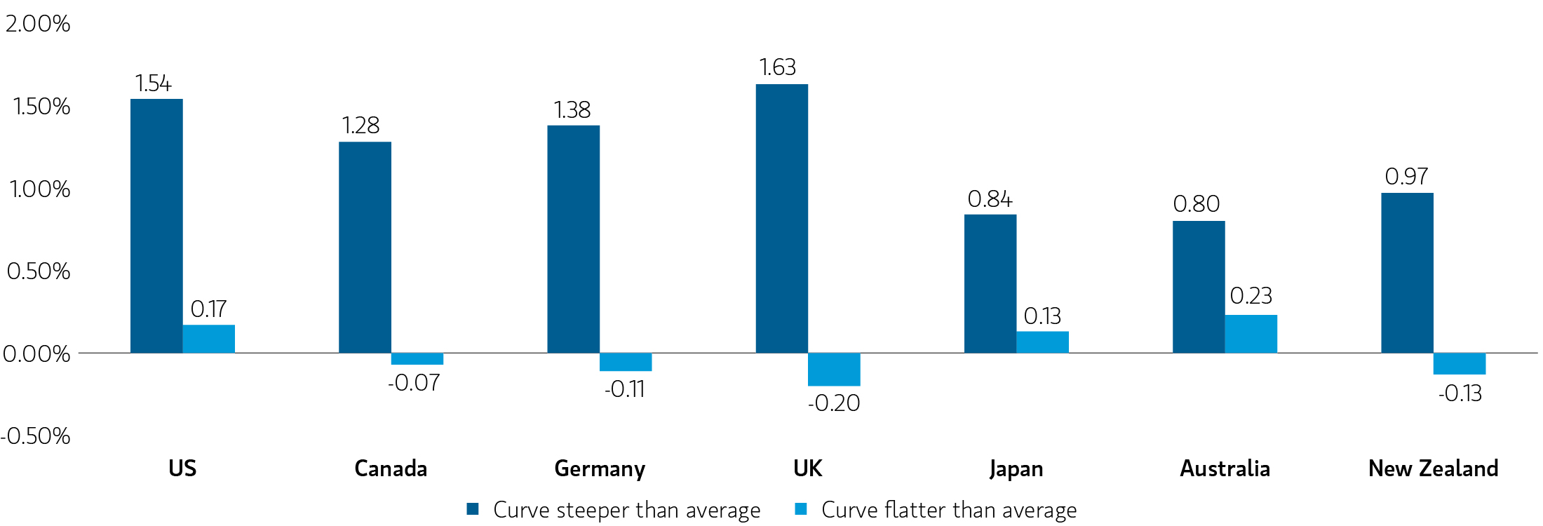
The shape of the yield curve is meant to reflect expectations for the future path of short‑term interest rates, with a steep curve signalling expected central bank tightening. In theory, one should not earn higher returns simply because the curve is steep: the gains from higher carry ought to be offset by capital losses as yields rise. In practice, however, excess returns have been higher when the curve is steeper than average, and lower when it is flatter. For USTs, average returns have been 1.54% when the curve is above‑average steepness and 0.17% when it is below average. This rule of thumb holds across DM rates (see Display 3). A common explanation for the success of carry in government bonds is that the curve is partly driven by term premium, and term premia tend to be larger when the curve is unusually steep.⁹

Display 3: Excess bond returns when yield curve is steep or flat

Source: MSIM, Bloomberg. Period of observation is 1997-2025. The indexes are provided for illustrative purposes only and are not meant to depict the performance of a specific investment. Past performance is no guarantee of future results.

Signal 5: Valuation

Our final principle is straightforward: purchase bonds when they are “cheap” and sell them when they are “rich.” Although value investing is a very intuitive and popular strategy in many markets, it has faced significant challenges in government bond markets in recent years. In particular, the use of unconventional monetary policy measures, such as Quantitative Easing, kept government bond yields at extraordinarily low levels for extended periods of time in the 2010s, which was then followed by a sharp rise in yields due to the inflation shock to the global economy following the Covid epidemic. Defining “value” in this context, in a way that helped one make successful investment decisions, has been challenging.

We therefore use a relatively simple measure of value: the current real yield on 10-year bonds relative to its 5-year average. Using real yields is intuitive, as it gives one an indication of the real return a long term investor should expect to receive. By adjusting it for its recent trading range helps adjust for the regime shifts we have seen over time, in both the economy and the central bank response function.

Constructing a Diversified Portfolio of Signals

The five signals above capture key drivers of government bond returns, which, when combined into one Quantitative Duration Strategy, leads to a reliable duration-positioning indicator, which enhances portfolio value over time.

We look to create a strategy which is balanced not only in terms of its data input but also how it performs. Some of the factors have a trending bias, e.g. Momentum suggests the more bonds sell off, the more one wants to short them; similarly for Risk Sentiment, the better the equities do, the more one should keep selling risk-free assets. On the other hand, valuation metrics (Valuation and Carry) provide a counterbalance to this, flagging when the rally or sell-off has gone too far[10].

The combination of five factors helps one identify high conviction investment opportunities, when valuations are still extreme but have started to correct back towards “fair value”.

This principle applies more broadly to the heuristics discussed and to the way we combine them to construct a more robust duration‑positioning indicator. Considered individually, each rule has limited utility in forecasting future returns; taken together, however, they can provide a more powerful and reliable signal. This is because each rule contributes a distinct, relevant perspective, yielding a more comprehensive view of likely interest‑rate dynamics. In effect, we assemble a diversified portfolio of fixed‑income signals, enhancing the resilience and overall quality of our investment approach.

For each rule, we derive a normalised signal on a common scale from -10 (most bearish, i.e., forecasting higher yields) to +10 (most bullish, i.e., forecasting lower yields). The composite positioning signal is calculated as the arithmetic average of the individual signals. To avoid acting on low‑conviction indications, we apply a neutral band around zero: if the composite score lies between -1.5 and +1.5, we set it to zero and refrain from taking a position. Throughout, we deliberately keep the indicator’s construction simple and transparent to facilitate interpretability and to mitigate the risk of data‑mining.

Limitations
QDS is built on well-researched inputs and readily available data, and its results have shown consistency across different market regimes. However, there are several limitations to consider:

Transaction costs
The results presented do not account for transaction costs. Yet we believe QDS performance can be replicated in real portfolios, particularly when investors express views via synthetic markets or transact in more liquid baskets. Additionally, setting the combined signal to neutral when it falls between -1.5 and +1.5 helps minimise trading frequency, reducing costs and noise.

Signal weights
As market conditions evolve, certain factors may outperform others, raising questions about factor weights and need for frequent rebalancing. Similarly, QDS can experience long periods of low-conviction scores, meaning it cannot always be relied upon to provide active investment recommendations. Since QDS is designed to inform fundamentally driven investment team rather than operate as a standalone strategy, we maintain equal weights for simplicity and transparency. This approach facilitates discussion on whether specific signals are better suited to prevailing market conditions.

Correlation between signals
Technical signal exhibits higher correlation with Risk Sentiment, which can reduce the efficacy of QDS output. On the other hand, relatively faster-moving Technical and Risk Sentiment signals show low or negative correlation to slower-moving Business Cycle, Carry and Value signals, providing a balanced mix of inputs.

Conclusion
Our proprietary MSIM Quantitative Duration Strategy (QDS) model advises us on tactical duration risk positioning in developed government bond markets over short time horizon (one to three months). The model is based on five signals incorporating both fundamental and technical inputs. Individually, these signals have limited predictive power for short-term government bond excess returns, but when combined they create a more robust and reliable signal. QDS has generated attractive Sharpe Ratios, strong performances during periods of market stress, and few significant drawdowns (before taking transaction costs into account).

Bibliography

Asness C.S., Moskowitz T.J., Pedersen L.H., (2013), Value and Momentum Everywhere, The Journal of Finance, Vol. 68, No. 3

Barberis N., Shleifer A., Vishny R., (1998), A model of investor, Journal of Financial Economics, Vol. 49, No. 3

De Long J.B., Shleifer A., Summers L.H., Waldmann R.J., (1990), Noise Trader Risk in Financial Markets, Journal of Political Economy, Vol. 98, No. 4

Hong, H. and Stein, J.C. (1999), A Unified Theory of Underreaction, Momentum Trading, and Overreaction in Asset Markets. The Journal of Finance, Vol. 54, No. 6

Ilmanen A. (1995), Time-Varying Expected Returns in International Bond Markets. The Journal of Finance, Vol. 50, No. 2

Ilmanen A., (1997), Forecasting US Bond Returns, The Journal of Fixed Income, Summer, 7 (1) pp 22-37

Ilmanen & Sayood (2002), “Quantitative Forecasting Models and Active Diversification for International Bonds”

Moskowitz T.J., Ooi Y.H., Pedersen L.H., (2012), Time series momentum, Journal of Financial Economics, Vol.104, No. 2

¹ Source: MSIM. Based on monthly data from January 1970 to June 2026

² Another way to address this issue would be through altering the weights assigned to each factor, depending on the regime one is in and/or the factor’s success, but we have not yet found a robust, systematic manner in which to do this.

³ Excess returns are government bond returns less the returns on T-bills. We use excess returns because it takes into account fixed income investors’ opportunity cost: there is no reason to hold bonds if they are expected to return less than cash. For leveraged investors it captures the cost of funding a bond position.

⁴ There is no fundamental justification for momentum as a QDS model investment factor. However, it is so widely documented across multiple asset classes that we are inclined to use it. Explanations for it tend to be behavioural in nature due to investors under- or over-reacting to new information (e.g. DeLong, Shleifer & Waldmann (1990); Barberis, Shleifer and Vishny (1998) and Hong & Stein (1999)), or due to hedging activity (e.g. Moskowitz, Ooi & Pedersen (2012)). In our experience, many of the largest fixed income investors (e.g. banks, insurers and pension funds) can be very slow-moving, and also invest for reasons other than the short-term maximising of expected returns (meeting regulatory requirements, hedging liabilities, etc.). It therefore seems plausible to us that there can be persistent flows in fixed income markets which can generate price momentum.

⁵ This is the explanation offered by Ilmanen (1995), who first observed that equity performance could be used to forecast bond returns.

⁶ Morgan Stanley, “MS Global Risk Demand Index”, Strategy and Economics, May 2004.

⁷ Our finding is consistent with “Quantitative Forecasting Models and Active Diversification for International Bonds” by Ilmanen & Sayood (2002).

⁸ Note that “duration carry” risk is very different in nature from “credit carry” risk (i.e. the additional yield investors are paid for taking on default risk) in two ways. First, its returns are more normally distributed, in contrast to credit risk which spikes lower when a default threatens. Second, it tends to be negatively correlated with risky asset returns, as the curve is steeper when the macroeconomic outlook is negative and the central bank has cut rates. This makes it a generally more attractive exposure to hold in a portfolio context.

⁹ If there is more term premium in the curve, it also implies that investors perceive there is more risk in being long duration. We look to address this in our QDS indicator by looking at volatility-adjusted returns, as the attraction of being long for carry partly depends on the risk associated with holding the position while one accrues the carry. This adjustment is of crucial importance when considering markets which have undergone regime shifts, e.g. the carry from owning Japanese Government Bonds (JGBs) is considerably lower than it was 20 years ago, but expected volatility has also collapsed. As a result, carry strategies can still be attractive even if the curve is a lot flatter now than it has been in the past.

¹⁰ “Value and Momentum Everywhere” by Asness, Moskowitz & Pedersen (2013) explores how the negative correlation between value and momentum investing leads to very effective combined investing strategies due to the negative correlation between the two strategies, and how this approach works well in multiple asset classes.

Broad Markets Fixed Income Team

Our team provides exposure to what we consider the best ideas in fixed income. Leveraging the expertise of our specialized teams, we use a team-based, rigorous and disciplined process that seeks out superior and repeatable results.

The Authors

Featured Insights

Viewed

Article

The MSIM Quantitative Duration Strategy Model: A Factor-Based Approach to Managing Interest Rates

Anton Heese and Matas Vala explore the Quantitative Duration Strategy Model, one of the proprietary tools the team uses to enhance their investment process, as it helps provide structure and rigour with identifying and processing relevant and important data.

05 August 2026

Viewed

Tales From the Emerging World

From Electric Vehicles to Humanoids: China’s Next Manufacturing Leap

Humanoid robots sit at the intersection of hardware, AI, manufacturing, real-world data and customer integration. Longer-term value may depend more on intelligence, software and fleet learning. Jerry Pang and Rose Kim examine how China’s humanoid robots are beginning to move from televised spectacles to manufacturing and commercial roles.

05 August 2026

Viewed

Quarterly

The BEAT™ for Q3 2026 - August

Use The BEAT™ as your timely resource for the markets. Each edition gives you ideas and insights that show you how to navigate the current investment environment.

05 August 2026

Viewed

Consilient Observer

The Wisdom of Crowds in Markets: Crowd Behavior in Prediction, Betting, and Stock Markets

We review the wisdom of crowds in the context of prediction markets, sports betting markets, parimutuel betting markets, and the stock market. For each, we describe the market, give a history, examine its accuracy, see how it aggregates information, check for diversity breakdowns, and consider the role of incentives. The betting markets are zero-sum, but the stock market has positive expected returns. Understanding how markets work is useful for evaluating opportunities for excess returns.

05 August 2026

Risk Considerations
Diversification does not eliminate the risk of loss. The value of investments held by the portfolio may increase or decrease in response to economic, and financial events (whether real, expected or perceived) in the U.S. and global markets. As interest rates rise, the value of certain income investments is likely to decline. Investments in debt instruments may be affected by changes in the creditworthiness of the issuer and are subject to the risk of non-payment of principal and interest. The value of income securities also may decline because of real or perceived concerns about the issuer’s ability to make principal and interest payments. U.S. Treasury securities generally have a lower return than other obligations because of their higher credit quality and market liquidity. While certain U.S. Government-sponsored agencies may be chartered or sponsored by acts of Congress, their securities are neither issued nor guaranteed by the U.S. Treasury. Investments rated below investment grade (sometimes referred to as “junk”) are typically subject to greater price volatility and illiquidity than higher rated investments. Investments in foreign instruments or currencies can involve greater risk and volatility than U.S. investments because of adverse market, economic, political, regulatory, geopolitical, currency exchange rates or other conditions. In the event of a default by a sovereign entity, there are typically no assets to be seized or cash flows to be attached. The portfolio is exposed to liquidity risk when trading volume, lack of a market maker or trading partner, large position size, market conditions, or legal restrictions impair its ability to sell particular investments or to sell them at advantageous market prices.

There is no guarantee that any investment strategy will work under all market conditions, and each investor should evaluate their ability to invest for the long-term, especially during periods of downturn in the market.

A separately managed account may not be appropriate for all investors. Separate accounts managed according to the Strategy include a number of securities and will not necessarily track the performance of any index. Please consider the investment objectives, risks and fees of the Strategy carefully before investing. A minimum asset level is required.

For important information about the investment managers, please refer to Form ADV Part 2.

The views and opinions and/or analysis expressed are those of the author or the investment team as of the date of preparation of this material and are subject to change at any time without notice due to market or economic conditions and may not necessarily come to pass. Furthermore, the views will not be updated or otherwise revised to reflect information that subsequently becomes available or circumstances existing, or changes occurring, after the date of publication. The views expressed do not reflect the opinions of all investment personnel at Morgan Stanley Investment Management (MSIM) and its subsidiaries and affiliates (collectively “the Firm”), and may not be reflected in all the strategies and products that the Firm offers.

Forecasts and/or estimates provided herein are subject to change and may not actually come to pass. Information regarding expected market returns and market outlooks is based on the research, analysis and opinions of the authors or the investment team. These conclusions are speculative in nature, may not come to pass and are not intended to predict the future performance of any specific strategy or product the Firm offers. Future results may differ significantly depending on factors such as changes in securities or financial markets or general economic conditions.

This material has been prepared on the basis of publicly available information, internally developed data and other third-party sources believed to be reliable. However, no assurances are provided regarding the reliability of such information and the Firm has not sought to independently verify information taken from public and third-party sources.

This material is a general communication, which is not impartial and all information provided has been prepared solely for informational and educational purposes and does not constitute an offer or a recommendation to buy or sell any particular security or to adopt any specific investment strategy. The information herein has not been based on a consideration of any individual investor circumstances and is not investment advice, nor should it be construed in any way as tax, accounting, legal or regulatory advice. To that end, investors should seek independent legal and financial advice, including advice as to tax consequences, before making any investment decision.

Charts and graphs provided herein are for illustrative purposes only. Past performance is no guarantee of future results.

This material is not a product of Morgan Stanley’s Research Department and should not be regarded as a research material or a recommendation.

The Firm has not authorised financial intermediaries to use and to distribute this material, unless such use and distribution is made in accordance with applicable law and regulation. Additionally, financial intermediaries are required to satisfy themselves that the information in this material is appropriate for any person to whom they provide this material in view of that person’s circumstances and purpose. The Firm shall not be liable for, and accepts no liability for, the use or misuse of this material by any such financial intermediary.

This material may be translated into other languages. Where such a translation is made this English version remains definitive. If there are any discrepancies between the English version and any version of this material in another language, the English version shall prevail.

The whole or any part of this material may not be directly or indirectly reproduced, copied, modified, used to create a derivative work, performed, displayed, published, posted, licensed, framed, distributed or transmitted or any of its contents disclosed to third parties without the Firm’s express written consent. This material may not be linked to unless such hyperlink is for personal and non-commercial use. All information contained herein is proprietary and is protected under copyright and other applicable law.

Morgan Stanley Investment Management is the asset management division of Morgan Stanley.

DISTRIBUTION
This material is only intended for and will only be distributed to persons resident in jurisdictions where such distribution or availability would not be contrary to local laws or regulations.

MSIM, the asset management division of Morgan Stanley (NYSE: MS), and its affiliates have arrangements in place to market each other’s products and services. Each MSIM affiliate is regulated as appropriate in the jurisdiction it operates. MSIM’s affiliates are: Calvert Research and Management, Eaton Vance Management, Parametric Portfolio Associates LLC, Parametric SAS, and Atlanta Capital Management LLC.

This material has been issued by any one or more of the following entities:

EMEA
This material is for Professional Clients/Accredited Investors only.

In the EU, MSIM materials are issued by MSIM Fund Management (Ireland) Limited (“FMIL”). FMIL is regulated by the Central Bank of Ireland and is incorporated in Ireland as a private company limited by shares with company registration number 616661 and has its registered address at 24-26 City Quay, Dublin 2, DO2 NY19, Ireland.

Outside the EU, MSIM materials are issued by Morgan Stanley Investment Management Limited (MSIM Ltd) is authorised and regulated by the Financial Conduct Authority. Registered in England. Registered No. 1981121. Registered Office: 25 Cabot Square, Canary Wharf, London E14 4QA.

In Switzerland, MSIM materials are issued by Morgan Stanley & Co. International plc, London (Zurich Branch) Authorised and regulated by the Eidgenössische Finanzmarktaufsicht (“FINMA”). Registered Office: Beethovenstrasse 33, 8002 Zurich, Switzerland.

Italy: MSIM FMIL (Milan Branch), (Sede Secondaria di Milano) Palazzo Serbelloni Corso Venezia, 16 20121 Milano, Italy. The Netherlands: MSIM FMIL (Amsterdam Branch), Rembrandt Tower, 11th Floor Amstelplein 1 1096HA, Netherlands. France: MSIM FMIL (Paris Branch), 61 rue de Monceau 75008 Paris, France. Spain: MSIM FMIL (Madrid Branch), Calle Serrano 55, 28006, Madrid, Spain. Germany: MSIM FMIL Frankfurt Branch, Große Gallusstraße 18, 60312 Frankfurt am Main, Germany (Gattung: Zweigniederlassung (FDI) gem. § 53b KWG). Denmark: MSIM FMIL (Copenhagen Branch), Gorrissen Federspiel, Axel Towers, Axeltorv2, 1609 Copenhagen V, Denmark.

MIDDLE EAST
Dubai International Financial Centre: This information does not constitute or form part of any offer to issue or sell, or any solicitation of any offer to subscribe for or purchase, any securities or investment products in the UAE (including the Dubai International Financial Centre and the Abu Dhabi Global Market) and accordingly should not be construed as such. Furthermore, this information is being made available on the basis that the recipient acknowledges and understands that the entities and securities to which it may relate have not been approved, licensed by or registered with the UAE Central Bank, the Dubai Financial Services Authority, the UAE Securities and Commodities Authority, the Financial Services Regulatory Authority or any other relevant licensing authority or government agency in the UAE. The content of this report has not been approved by or filed with the UAE Central Bank, the Dubai Financial Services Authority, the UAE Securities and Commodities Authority or the Financial Services Regulatory Authority.

Abu Dhabi Global Market (“ADGM”): This material is sent strictly within the context of, and constitutes, an Exempt Communication. This material relates to the strategy which is not subject to any form of regulation or approval by the Financial Services Regulatory Authority of the Abu Dhabi Global Market (the “FSRA”).

Saudi Arabia
This financial promotion was issued and approved for use in Saudi Arabia by Morgan Stanley Saudi Arabia, Al Rashid Tower, Kings Sand Street, Riyadh, Saudi Arabia, authorized and regulated by the Capital Market Authority license number 06044-37.

U.S. NOT FDIC INSURED. OFFER NO BANK GUARANTEE. MAY LOSE VALUE. NOT INSURED BY ANY FEDERAL GOVERNMENT AGENCY.NOT A DEPOSIT.

Latin America (Brazil, Chile Colombia, Mexico, Peru, and Uruguay) This material is for use with an institutional investor or a qualified investor only. All information contained herein is confidential and is for the exclusive use and review of the intended addressee, and may not be passed on to any third party. This material is provided for informational purposes only and does not constitute a public offering, solicitation or recommendation to buy or sell for any product, service, security and/or strategy. A decision to invest should only be made after reading the strategy documentation and conducting in-depth and independent due diligence.

ASIA PACIFIC
Hong Kong: This document has been issued by Morgan Stanley Asia Limited, CE No. AAD291, for use in Hong Kong and shall only be made available to “professional investors” as defined under the Securities and Futures Ordinance of Hong Kong (Cap 571). The contents of this document have not been reviewed nor approved by any regulatory authority including the Securities and Futures Commission in Hong Kong. Accordingly, save where an exemption is available under the relevant law, this document shall not be issued, circulated, distributed, directed at, or made available to, the public in Hong Kong. Singapore: This material is disseminated in Singapore by Morgan Stanley Investment Management Company, Registration No. 199002743C. This material should not be considered to be the subject of an invitation for subscription or purchase, whether directly or indirectly, to the public or any member of the public in Singapore other than (i) to an institutional investor under section 304 of the Securities and Futures Act, Chapter 289 of Singapore (“SFA”), (ii) to a “relevant person” (which includes an accredited investor) pursuant to section 305 of the SFA, and such distribution is in accordance with the conditions specified in section 305 of the SFA; or (iii) otherwise pursuant to, and in accordance with the conditions of, any other applicable provision of the SFA. This material has not been reviewed by the Monetary Authority of Singapore. Australia: This material is provided by Morgan Stanley Investment Management (Australia) Pty Ltd ABN 22122040037, AFSL No. 314182 and its affiliates and does not constitute an offer of interests. Morgan Stanley Investment Management (Australia) Pty Limited arranges for MSIM affiliates to provide financial services to Australian wholesale clients. This material will not be lodged with the Australian Securities and Investments Commission.

Japan
For professional investors, this material is circulated or distributed solely for informational purposes. For non-professional investors, this material is provided in connection with Morgan Stanley Investment Management (Japan) Co., Ltd. (“MSIMJ”)’s business with respect to discretionary investment management agreements (“IMA”) and investment advisory agreements (“IAA”). This does not constitute a recommendation or solicitation of transactions nor offers any particular financial instruments. Under an IMA, with respect to the management of client assets, the client prescribes basic management policies in advance and commissions MSIMJ to make all investment decisions based on an analysis of the value, etc. of the securities, and MSIMJ accepts such commission. The client shall delegate to MSIMJ the authorities necessary to make such investment decisions. MSIMJ exercises these delegated authorities accordingly, and the client shall not make individual instructions. All investment profits and losses belong to the clients; principal is not guaranteed. Please consider the investment objectives and nature of risks before investing. As an investment advisory fee for an IAA or an IMA, the amount of assets subject to the contract multiplied by a certain rate (the upper limit is 2.20% per annum (including tax)) shall be incurred in proportion to the contract period. For some strategies, a contingency fee may be incurred in addition to the fee mentioned above. Indirect charges also may be incurred, such as brokerage commissions for underlying securities. Since these charges and expenses vary by contract and other factors, MSIMJ cannot present the rates, upper limits, etc. in advance. All clients should read thoroughly the Documents Provided Prior to the Conclusion of a Contract carefully before executing an agreement. This material is distributed in Japan by MSIMJ, Registered No. 410 (Director of Kanto Local Finance Bureau (Financial Instruments Firms)), Membership: the Japan Securities Dealers Association, the Investment Management Association of Japan and the Type II Financial Instruments Firms Association.

For professional investors, this material is circulated or distributed for informational purposes only. For those who are not professional investors, this material is provided in relation to Morgan Stanley Investment Management (Japan) Co., Ltd. (“MSIMJ”)’s business with respect to discretionary investment management agreements (“IMA”) and investment advisory agreements (“IAA”). This is not for the purpose of a recommendation or solicitation of transactions or offers any particular financial instruments. Under an IMA, with respect to management of assets of a client, the client prescribes basic management policies in advance and commissions MSIMJ to make all investment decisions based on an analysis of the value, etc. of the securities, and MSIMJ accepts such commission. The client shall delegate to MSIMJ the authorities necessary for making investment. MSIMJ exercises the delegated authorities based on investment decisions of MSIMJ, and the client shall not make individual instructions. All investment profits and losses belong to the clients; principal is not guaranteed. Please consider the investment objectives and nature of risks before investing. As an investment advisory fee for an IAA or an IMA, the amount of assets subject to the contract multiplied by a certain rate (the upper limit is 2.20% per annum (including tax)) shall be incurred in proportion to the contract period. For some strategies, a contingency fee may be incurred in addition to the fee mentioned above. Indirect charges also may be incurred, such as brokerage commissions for incorporated securities. Since these charges and expenses are different depending on a contract and other factors, MSIMJ cannot present the rates, upper limits, etc. in advance. All clients should read the Documents Provided Prior to the Conclusion of a Contract carefully before executing an agreement. This material is disseminated in Japan by MSIMJ, Registered No. 410 (Director of Kanto Local Finance Bureau (Financial Instruments Firms)), Membership: the Japan Securities Dealers Association, The Investment Trusts Association, Japan, the Japan Investment Advisers Association and the Type II Financial Instruments Firms Association.